Ebola example - using EpiEstim for estimation
epiestim_ebola.Rmd
library(EpiControl)
library(VGAM)
library(parallel)
library(pbapply)
library(zoo)  # For rolling sum operations
library(ggplot2)
library(EpiEstim)

library(readr)
library(dplyr)
library(tidyr)
set.seed(1)Data preprocessing
We will first load the dataset containing cases of West African Ebola. Garske, T. et al. Heterogeneities in the case fatality ratio in the West African Ebola outbreak 2013–2016. Philos. Trans. R. Soc. Lond. B Biol. Sci. 372, 20160308 2017. link
# Read data
ebola_data <- read_csv("ebola_data/rstb20160308_si_001.csv")

# Extract and convert date column
date_reported <- as.Date(ebola_data$DateReport)  # Ensure it's in Date format
date_inferred <- as.Date(ebola_data$DateOnsetInferred)

# Create a sequence of all dates from min to max
all_dates <- data.frame(date_reported = seq(min(date_reported, na.rm = TRUE),
                                            max(date_reported, na.rm = TRUE),
                                            by = "day"))

# Count occurrences of each reported date
date_counts <- as.data.frame(table(date_reported, useNA = "no"))
date_counts_i <- as.data.frame(table(date_inferred, useNA = "no"))

colnames(date_counts) <- c("date_reported", "count")
colnames(date_counts_i) <- c("date_reported", "count")
date_counts$date_reported <- as.Date(date_counts$date_reported)
date_counts_i$date_reported <- as.Date(date_counts_i$date_reported)# Convert back to Date format

# Merge full date range with counts, filling missing dates with 0
date_counts_filled <- all_dates %>%
  left_join(date_counts, by = "date_reported") %>%
  replace_na(list(count = 0))

date_counts_i_filled <- all_dates %>%
  left_join(date_counts_i, by = "date_reported") %>%
  replace_na(list(count = 0))

date_counts_filled$count_i <- date_counts_i_filled$count

# Visualise daily epidemic cases curves (when reported and as occurence inferred)

ggplot(date_counts_filled, aes(x = date_reported, y = count)) +
  geom_line(color = "blue") +  # Line plot for cases over time
  geom_line(color = "red", aes(x = date_reported, y = count_i)) +
  labs(title = "Ebola Cases Over Time",
       x = "Date",
       y = "Number of Cases") +
  theme_minimal()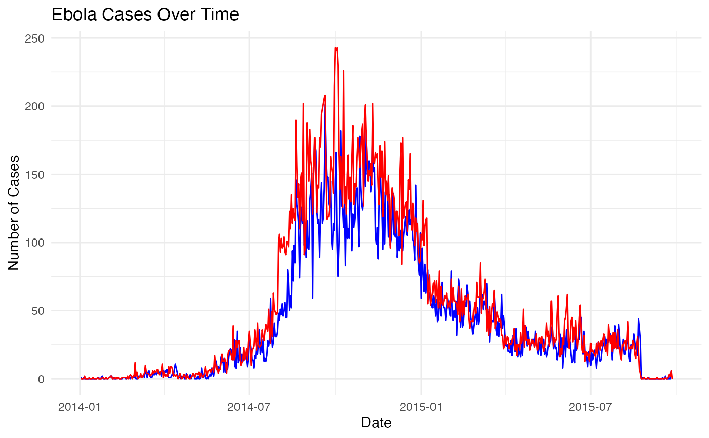
Let’s estimate R from this data using EpiEstim.
cases_v <- date_counts_filled$count_i

ndays <- 833#epidemic length #simulation length

# Assumed generation time distribution
Ygen <- dgamma(1:ndays, 15.0/2.1, 1/2.1)
Ygen <- Ygen/sum(Ygen)
Ygen <- c(0, Ygen)

res <- estimate_R(incid = cases_v,
                  method = "non_parametric_si",
                  config = make_config(si_distr = Ygen))


plot(res)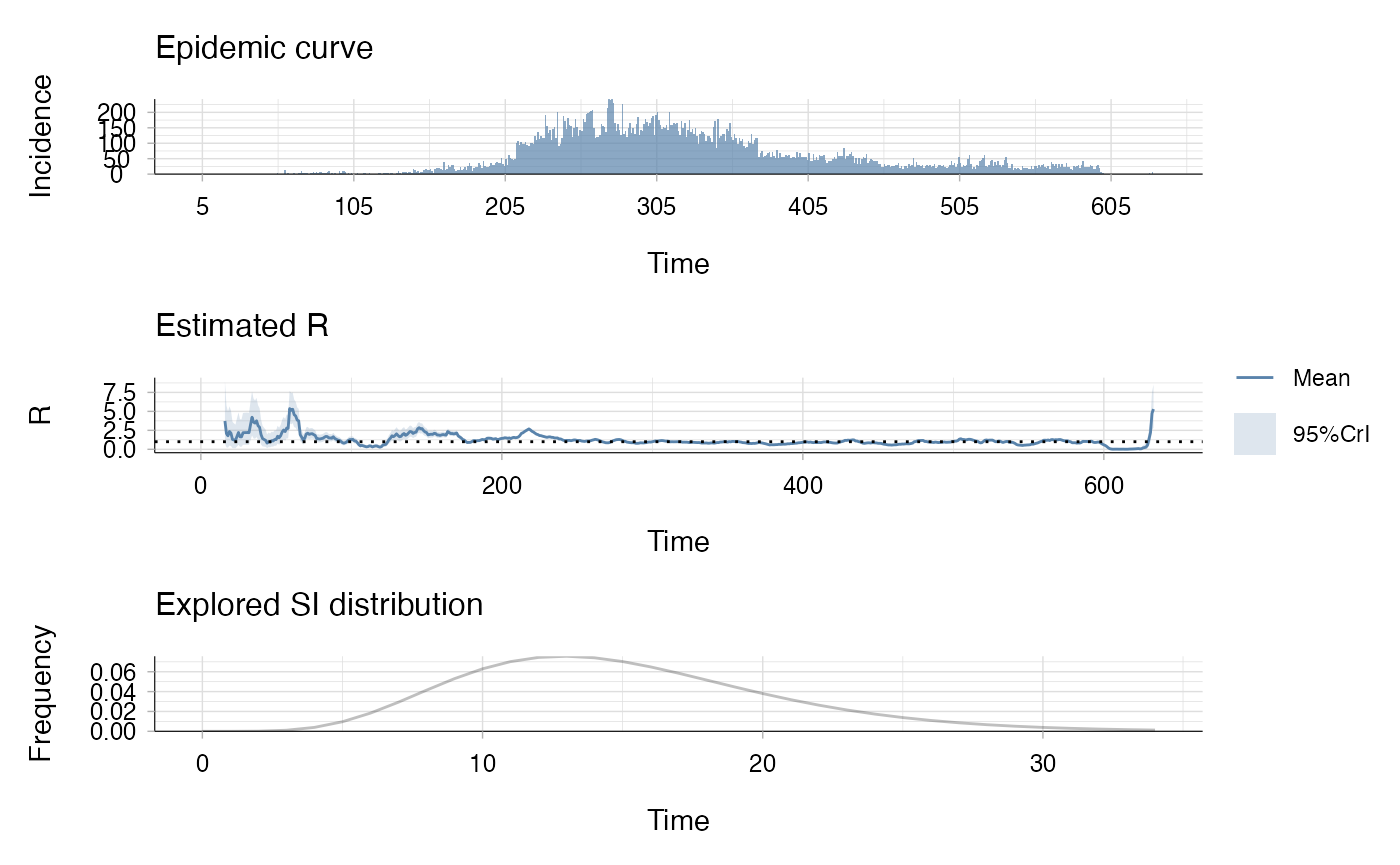
Simulation setup
We simulate a controlled epidemic starting on day 210 after the first case. We will set the control target to 50 cases/day. We will model susceptible depletion by infected individuals getting removed from the susceptible group. We expect the control to balance cases around the target until herd immunity is reached and then no further interventions applied.
Initialise the cluster for parallel computing:
cores <- detectCores() - 1
cl <- makeCluster(cores)

clusterSetRNGStream(cl, iseed = 20250501)
Define the epidemic ans noise parameters
We will use pathogen = 2 corresponding to Ebola Virus Disease.
Epi_pars <- data.frame(
  Pathogen = c("COVID-19", "Ebola"),
  R0 = c(1.305201/0.5, 2.5),
  gen_time = c(6.5, 15.0),
  gen_time_var = c(2.1, 2.1),
  CFR = c(0.0132, 0.5),
  mortality_mean = c(10.0, 10.0),
  mortality_var = c(1.1, 1.1)
)

Noise_pars <- data.frame(
  repd_mean = 10.5,  # Reporting delay mean
  del_disp = 5.0,    # Reporting delay variance
  ur_mean = 0.3,     # Under-reporting mean
  ur_beta_a = 50.0   # Beta distribution alpha for under-reporting
)
Action Space for Policy Interventions
Define non-pharmaceutical interventions: We have 3 actions, introducing a lockdown, social distancing and no interventions.
# Setting-up the control (using non-pharmaceutical interventions)
Action_space <- data.frame (
  NPI = c("No restrictions", "Social distancing", "Lockdown"),
  R_coeff = c(1.0, 0.7, 0.4), #R0_act = R0 * ctrl_states
  R_beta_a = c(0.0, 5.0, 5.0), #R0_act uncertainty
  cost_of_NPI = c(0.0, 0.01, 0.15)
)
Simulation parameters
We set the simulation parameters, targets, R estimation window etc. below. We do not account for vaccination or new variants, therefore we set v_max_rate = 0 and delta_multiplier = 1.0.
N <- 1e6 # population size
I0 <- 10 # initial infections
real_days <- 210L #we start the simulation from data here

#Simulation parameters
n_ens <- 20L #MC assembly size for 4
sim_ens <- 20L #assembly size for full simulation

C_target <- 50
D_target <- 25
r_trans_len <- 7

sim_settings <- list(
  ndays = ndays, #simulation length
  start_day = real_days,
  N = N, # population size
  I0 = I0, # initial infections
  C_target = C_target, #target cases
  C_target_pen = C_target*1.5, #overshoot penalty threshold
  R_target = 1.0,
  D_target = D_target, #one way to get peaks at 400 is to increase this to 15
  D_target_pen = 50, #max death
  #alpha = 1.3/C_target, #~proportional gain (regulates error in cases) covid
  alpha = 3.25/C_target, #~proportional gain (regulates error in cases) ebola
  alpha_d = 0*1.3/D_target,
  ovp = 5.0, #overshoot penalty
  dovp = 0*10.0, #death overshoot penalty
  gamma = 0.95, #discounting factor
  n_ens = n_ens, #MC assembly size for 4
  sim_ens = sim_ens, #assembly size for full simulation
  rf = 14L, #days 14
  R_est_wind = 5L, #rf-2 #window for R estimation
  pred_days = 21L,
  r_trans_steep = 1.5,  # Growth rate
  r_trans_len = r_trans_len,  # Number of days for the transition
  t0 = r_trans_len  / 2, # Midpoint of the transition
  pathogen = 2,
  susceptibles = 1,
  delay = 1,
  ur = 1,
  r_dir = 2,
  LD_on = 14, #on threshold
  LD_off = 7, #off threshold
  v_max_rate = 0,
  vac_scale = 100,
  vac_start = 370,
  delta_scale = 40,
  delta_start = 550,
  delta_multiplier = 1.0,
  v_protection_delta = (58+85)/200,
  v_protection_alpha = 0.83
)

# Construct our simulation dataframe:
column_names <- c("days", "sim_id", "I", "Lambda", "C", "Lambda_C", "S", "Re", "Rew", "Rest", "R0est", "policy", "R_coeff", "Real_C", "vaccination_rate", "delta_prevalence","immunity")

# Create an empty data frame with specified column names
empty_df <- data.frame(matrix(ncol = length(column_names), nrow = 0))
colnames(empty_df) <- column_names

# Create a zero matrix with 10 rows
zero_matrix <- matrix(0, nrow = ndays, ncol = length(column_names))
colnames(zero_matrix) <- column_names

# Combine empty data frame and zero matrix using rbind
episim_data <- rbind(empty_df, zero_matrix)

#initialisation

episim_data['policy'] <- rep(2, ndays)
episim_data['sim_id'] <- rep(1, ndays)
episim_data[1:real_days,] <- c(1, 1, I0, I0, Noise_pars['ur_mean']*I0, Noise_pars['ur_mean']*I0, N-I0, Epi_pars[1,'R0']*0.5, Epi_pars[1,'R0']*0.5, Epi_pars[1,'R0']*0.5, Epi_pars[1,'R0'], 2, 0.5, 0, 0, 0, 0)
episim_data['days'] <- 1:ndays
episim_data['date'] <- all_dates[1:ndays, 'date_reported']

episim_data[1:real_days,"C"] <- date_counts_filled$count_i[1:real_days]
episim_data[1:real_days,"I"] <- date_counts_filled$count_i[1:real_days]/0.3
episim_data[1:nrow(episim_data),"Real_C"] <- date_counts_filled$count_i[1:nrow(episim_data)]

# get infectiousness and estimated R-s

gen_time <- 15.0
gen_time_var <- 2.1

R_est_wind <- 5  # Define your window size

Ygen <- dgamma(1:nrow(ebola_data), gen_time/gen_time_var, 1/gen_time_var)
Ygen <- Ygen/sum(Ygen)

# Estimate R
for (ii in 1:real_days+1) {
  if (ii-1 < R_est_wind) {
    episim_data[ii, 'Rest'] <- mean(episim_data[1:(ii-1), 'C']) / mean(episim_data[1:(ii-1), 'Lambda_C'])
    R_coeff_tmp <- sum(Ygen[1:(ii-1)] * episim_data[(ii-1):1, 'R_coeff']) / sum(Ygen[1:(ii-1)])
  } else {
    if ( mean(episim_data[(ii-R_est_wind):(ii-1), 'Lambda_C']) == 0){
      episim_data[ii, 'Rest'] <- 0
      R_coeff_tmp <- 1
    } else {
      episim_data[ii, 'Rest'] <- mean(episim_data[(ii-R_est_wind):(ii-1), 'C']) / mean(episim_data[(ii-R_est_wind):(ii-1), 'Lambda_C'])
      R_coeff_tmp <- sum(Ygen[1:(ii-1)] * episim_data[(ii-1):1, 'R_coeff']) / sum(Ygen[1:(ii-1)])
    }
  }
  episim_data[ii, 'R0est'] <- episim_data[ii, 'Rest'] / R_coeff_tmp
  episim_data[ii, 'Lambda_C'] <- sum(episim_data[(ii-1):1,'C']*Ygen[1:(ii-1)])
  episim_data[ii, 'Lambda'] <- sum(episim_data[(ii-1):1,'I']*Ygen[1:(ii-1)])
}

Epi_pars[1,"R0"] <- episim_data[real_days, 'R0est']

episim_data_ens <- replicate(sim_ens, episim_data, simplify = FALSE)

for (ii in 1:sim_ens) {
  episim_data_ens[[ii]]$sim_id <- rep(ii, ndays)
}
Running the simulation
Passing the simulation setup to epicontrol and running the simulation.
episettings <- list(
  sim_function = Epi_MPC_run_V,
  reward_function = reward_fun,
  R_estimator = R_estim,
  noise_par = Noise_pars,
  epi_par = Epi_pars,
  actions = Action_space,
  sim_settings = sim_settings,
  parallel = TRUE
)

episim_data_ens <- replicate(sim_ens, episim_data, simplify = FALSE)

for (ii in 1:sim_ens) {
  episim_data_ens[[ii]]$sim_id <- rep(ii, ndays)
}

episettings$cl <- cl

results <- epicontrol(episim_data_ens, episettings)
#> [1] 1
#>   |                                                          |                                                  |   0%

episim_data_ens <- results
stopCluster(cl)

## For non-parallel runs:

#for (jj in 1:sim_ens) {
#  episim_data_ens[[jj]] <- Epi_MPC_run_wd(episim_data_ens[[jj]], Epi_pars, Noise_pars, Action_space, pred_days = pred_days, n_ens = n_ens, ndays = nrow(episim_data), R_est_wind = R_est_wind, pathogen = 1, susceptibles = 0, delay = 0, ur = 0, r_dir = 2, N = N)
#  setTxtProgressBar(pb,jj)
#}
#close(pb)

# Combine Simulation Results
combined_data <- do.call(rbind, episim_data_ens)
Plotting results
combined_data <- combined_data %>%
  group_by(sim_id, policy) %>%
  arrange(days) %>%
  mutate(group = cumsum(c(1, diff(days) != 1))) %>%
  ungroup()

combined_data <- combined_data %>%
  arrange(sim_id, days, policy)

policy_labels <- c("0" = "Historical data", "2" = "Social distancing", "3" = "Lockdown")

combined_data$policy[combined_data$days < real_days] <- 0

combined_data$date <- date_counts_i_filled[1, 'date_reported']  + (combined_data$days - 1)
# Assuming combined_data has a 'date' column
ggplot(combined_data %>% filter(sim_id == 1)) +
  geom_line(data = subset(combined_data, sim_id != 1),
            aes(x = date, y = C, color = as.factor(sim_id)), alpha = 0.1) +
  geom_line(aes(x = date, y = C, color = factor(policy, labels = policy_labels), group = 1), alpha = 1.0) +
  geom_line(aes(x = date, y = Real_C, color = "blue", group = 1), alpha = 1.0, size = 0.25) +
  geom_hline(yintercept = C_target, linetype = "dashed", color = "blue", size = 0.25) +
  geom_vline(xintercept = date_counts_i_filled[1, 'date_reported'] + (real_days - 1),
             linetype = "dashed", color = "black", size = 0.25) +
  labs(x = "Date", y = "Reported cases", color = "Policy") +
  scale_color_manual(values = c("No intervention" = "chartreuse3",
                                "Social distancing" = "darkorchid1",
                                "Lockdown" = "red",
                                "Historical data" = "black")) +
  guides(color = guide_legend(title = "Policy"))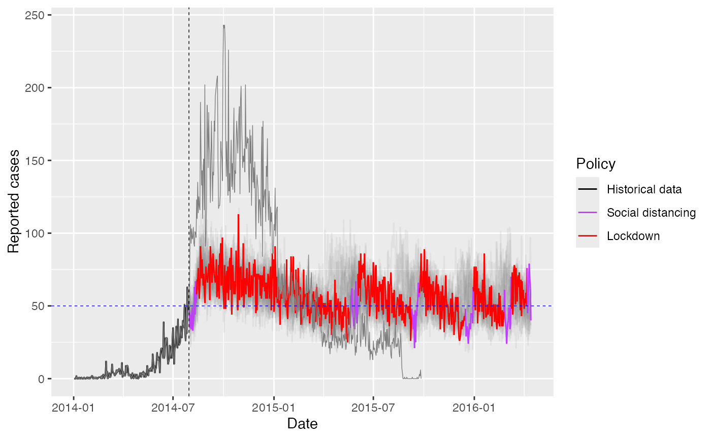
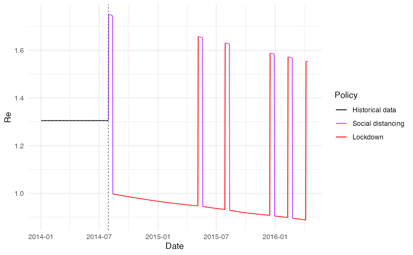
ggplot(combined_data %>% filter(sim_id == 2)) +
  geom_line(aes(x = date, y = Re, color = factor(policy, labels = policy_labels), group = 1), alpha = 1.0) +
  scale_color_manual(values = c("No intervention" = "chartreuse3",
                                "Social distancing" = "darkorchid1",
                                "Lockdown" = "red",
                                "Historical data" = "black")) +
  labs(x = "Date", y = "Re", color = "Policy") +
  guides(color = guide_legend(title = "Policy")) +
  geom_vline(xintercept = date_counts_i_filled[1, 'date_reported'] + (real_days - 1),
             linetype = "dashed", color = "black", size = 0.25) +
  theme_minimal()