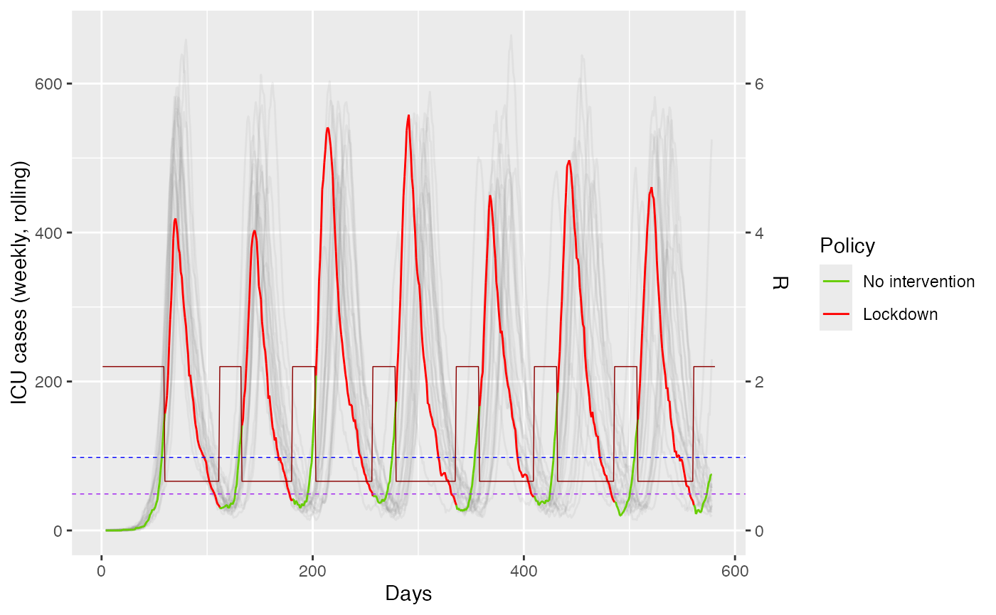
Threshold-based control of ICU cases for COVID-19

Overview

This vignette demonstrates threshold-based control of ICU cases for COVID-19

Load Libraries and Setup

Load the required libraries and initialize the simulation environment.

library(EpiControl)
library(VGAM)
library(parallel)
library(pbapply)
library(zoo)  # For rolling sum operations
library(dplyr)
library(ggplot2)

set.seed(1)

Initialize the cluster for parallel computing:

cores <- detectCores() - 1
cl <- makeCluster(cores)

clusterSetRNGStream(cl, iseed = 20250501)

Epidemiological and Noise Parameters

Define parameters for pathogens and noise: Can include different pathogens, in this case we consider COVID-19 and Ebola virus.

Epi_pars <- data.frame(
  Pathogen = c("COVID-19", "Ebola"),
  R0 = c(2.2, 2.5),
  gen_time = c(6.5, 15.0),
  gen_time_var = c(2.1, 2.1),
  CFR = c(0.0132, 0.5),
  mortality_mean = c(10.0, 10.0),
  mortality_var = c(1.1, 1.1)
)

Noise_pars <- data.frame(
  repd_mean = 10.5,  # Reporting delay mean
  del_disp = 5.0,    # Reporting delay variance
  ur_mean = 0.3,     # Under-reporting mean
  ur_beta_a = 50.0   # Beta distribution alpha for under-reporting
)

Action Space for Policy Interventions

Define non-pharmaceutical interventions: We have 2 actions, introducing a “lockdown” and no interventions.

Action_space <- data.frame(
  NPI = c("No restrictions", "Lockdown"),
  R_coeff = c(1.0, 0.3),
  R_beta_a = c(0.0, 5.0),
  cost_of_NPI = c(0.0, 0.15)
)

Simulation Setup

Set up key parameters and initialize simulation data:

r_trans_len <- 7

sim_settings <- list(
  ndays = 83 * 7, #simulation length
  start_day = 1,
  N = 1e7, # population size
  I0 = 10, # initial infections
  sim_ens = 20L, #assembly size for full simulation
  rf = 1L, #days 14
  R_est_wind = 5L, #rf-2 #window for R estimation
  r_trans_steep = 1.5,  # Growth rate
  r_trans_len = r_trans_len,  # Number of days for the transition
  t0 = r_trans_len  / 2, # Midpoint of the transition
  pathogen = 1,
  susceptibles = 0,
  delay = 0,
  ur = 0,
  r_dir = 2,
  LD_on = 14,
  LD_off = 7
)

column_names <- c("days", "sim_id", "I", "Lambda", "C", "Lambda_C", "S", "Deaths", "Re", "Rew", "Rest", "R0est", "policy", "R_coeff")
episim_data <- data.frame(matrix(0, nrow = (sim_settings$ndays), ncol = length(column_names)))
colnames(episim_data) <- column_names

episim_data$policy <- rep(1, sim_settings$ndays)
episim_data$days <- 1:(sim_settings$ndays)
episim_data[1, ] <- c(1, 1, sim_settings$I0, sim_settings$I0, Noise_pars$ur_mean * sim_settings$I0, Noise_pars$ur_mean * sim_settings$I0, sim_settings$N - sim_settings$I0, 0, Epi_pars[1, "R0"], Epi_pars[1, "R0"], 1, 1, 1, 1)

episim_data_ens <- replicate(sim_settings$sim_ens, episim_data, simplify = FALSE)

for (ii in 1:sim_settings$sim_ens) {
  episim_data_ens[[ii]]$sim_id <- rep(ii, sim_settings$ndays)
}

Running the Simulation

Run simulations in parallel using the pblapply function:

episettings <- list(
  sim_function = Epi_MPC_run_wd_thr,
  R_estimator = R_estim,
  noise_par = Noise_pars,
  epi_par = Epi_pars,
  actions = Action_space,
  sim_settings = sim_settings,
  parallel = TRUE
)

episettings$cl <- cl

results <- epicontrol(episim_data_ens, episettings)
#> [1] 0
#>   |                                                          |                                                  |   0%

episim_data_ens <- results
stopCluster(cl)

#for (jj in 1:sim_ens) {
#  episim_data_ens[[jj]] <- Epi_MPC_run_wd(episim_data_ens[[jj]], Epi_pars, Noise_pars, Action_space, pred_days = pred_days, n_ens = n_ens, ndays = nrow(episim_data), R_est_wind = R_est_wind, pathogen = 1, susceptibles = 0, delay = 0, ur = 0, r_dir = 2, N = N)
#  setTxtProgressBar(pb,jj)
#}
#close(pb)

for (jj in 1:sim_settings$sim_ens) {
  episim_data_ens[[jj]]["D_roll"] <- rollsum(episim_data_ens[[jj]]["Deaths"], 7, fill = NA)
  episim_data_ens[[jj]]["I_roll"] <- rollsum(episim_data_ens[[jj]]["I"], 7, fill = NA)
  episim_data_ens[[jj]]["D_cum"] <- cumsum(episim_data_ens[[jj]]["Deaths"])
  episim_data_ens[[jj]]["I_cum"] <- cumsum(episim_data_ens[[jj]]["I"])
}

# Combine Simulation Results
combined_data <- do.call(rbind, episim_data_ens)

Plotting results


combined_data <- combined_data %>%
  group_by(sim_id, policy) %>%
  arrange(days) %>%
  mutate(group = cumsum(c(1, diff(days) != 1))) %>%
  ungroup()

combined_data <- combined_data %>%
  arrange(sim_id, days, policy)

policy_labels <- c("1" = "No intervention", "2" = "Lockdown")


# Plotting the data
ggplot(combined_data %>% filter(sim_id == 1)) +
  geom_line(data = subset(combined_data, sim_id != 1), aes(x = days, y = D_roll, color = as.factor(sim_id)), alpha = 0.1) +
  geom_line(aes(x = days, y = D_roll, color = factor(policy, labels = policy_labels), group = 1), alpha = 1.0) +
  geom_line(aes(x = days, y = D_roll, color = factor(policy, labels = policy_labels), group = 1), alpha = 1.0, size=0.25) +
  geom_hline(yintercept = 7*sim_settings$LD_on, linetype = "dashed", color = "blue", size=0.25) +
  geom_hline(yintercept = 7*sim_settings$LD_off, linetype = "dashed", color = "purple", size=0.25) +
  labs(x = "Days", y = "Reported cases (rolling weekly", color = "Policy") +
  scale_color_manual(values = c("No intervention" = "chartreuse3", "Lockdown" = "red")) +
  guides(color = guide_legend(title = "Policy")) +
  scale_y_continuous(
    name = "ICU cases (weekly, rolling)",
    sec.axis = sec_axis(~./100, name = "R")
  ) +
  geom_line(data = subset(combined_data, sim_id == 1), aes(x = days, y = 100*Re), color = "darkred", size=0.25, alpha = 1.0)

Sandor Beregi