Use EpiControl with compartmental models
Sandor Beregi
2026-04-15
compartmental.RmdOverview
We will use the MPC algorithm with an SVIR model (SIR with vaccination), where we apply interventions reducing the transmission rate. Projections to evaluate the cost function are still made using a renewal model.
SVIR model description
We consider an event-based, stochastic compartmental SVIR epidemic model with four population groups:
- S: susceptible individuals
- V: vaccinated individuals
- II: infectious individuals
- R: recovered individuals
The total population size is fixed:
\[ N = S(t) + II(t) + R(t) + V(t). \]
The model assumes that susceptible individuals may either become vaccinated or infected. Infectious individuals recover at a constant per-capita rate. The vaccine provides full immunity (vaccinated individuals never get infected).
We introduce the model equations with the equilvalent (deterministic) ordinary differential equation system:
\[ \frac{dS}{dt} = - \beta \frac{S}{N} II - \nu S \]
\[ \frac{dII}{dt} = \beta \frac{S}{N} II - \gamma II \]
\[ \frac{dR}{dt} = \gamma II \]
\[ \frac{dV}{dt} = \nu S. \]
This means that:
- susceptible individuals leave \(S\) through either infection or vaccination,
- newly infected individuals enter \(II\),
- infectious individuals recover into \(R\),
- vaccinated individuals move into \(V\).
and \(\beta, \gamma\) and \(\nu\) are the infection, recovery and vaccination rates.
Stochastic event interpretation
In our implementation, infection, vaccination, and recovery are represented as event-driven transitions over each time step \(dt\). For susceptible individuals, infection and vaccination compete as alternative events, while recovery acts on the infectious compartment. The realised changes in each compartment are then aggregated into the state update.
The model records the following event counts at each step:
- Infections
- Vaccinations
- Recoveries
and the change of the compartment populations are given by
\[ \Delta S = -\text{Infections} - \text{Vaccinations} \] \[ \Delta V = \text{Vaccinations} \] \[ \Delta II = \text{Infections} - \text{Recoveries} \]
\[ \Delta R = \text{Recoveries} \]
Initialisation
library(EpiControl)
library(VGAM)
library(parallel)
library(pbapply)
library(zoo)  # For rolling sum operations
library(dplyr)
library(ggplot2)
set.seed(1)Let’s define model and surveillance noise parameter accounting for
epresent reporting delays and incomplete ascertainment in observed case
counts. We model reported cases \(C_t\)
as a noisy observation of the underlying infectious process \(I_t\). To account for reporting delays, the
expected number of reported cases at time \(t\) is constructed by convolving past
infectious counts with a delay distribution
Gamma(1:ndays, shape = gen_time / gen_time_var, rate = 1 / gen_time_var).
The delayed count is then observed through a Poisson sampling step
pois_input_c <- sum(episimdata[ii:1, 'I'] * Ydel[1:ii])
and C_del <- rpois(1, pois_input_c) . Optional
under-reporting is incorporated using a beta-binomial observation model
C <- VGAM::rbetabinom.ab(1, C_del, ur_beta_a, ur_beta_b)
with ur_beta_b <- (1 - ur_mean) / ur_mean * ur_beta_a,
applied either to the delayed count or, when no delay is included,
directly to \(I_t\).
Epi_pars <- data.frame(
  Pathogen = c("COVID-19"),
  R0 = c(2.8),
  sigma = c(1/6.5), #recovery rate
  vaccination_rate = c(1/1000), #vaccination rate
  gen_time = c(6.5), # for the renewal model used in projections
  gen_time_var = c(6.5), # for the renewal model used in projections
  CFR = c(0.0132), # case fatality ratio
  mortality_mean = c(10.0), # mean time from infection to death (for renewal model projections)
  mortality_var = c(1.1) # mean time from infection to death (for renewal model projections)
)

Noise_pars <- data.frame(
  repd_mean = 10.5,  # Reporting delay mean
  del_disp = 5.0,    # Reporting delay variance
  ur_mean = 0.3,     # Under-reporting mean
  ur_beta_a = 50.0   # Beta distribution alpha for under-reporting
)
Simulation/model projection parameters and cost function
We choose the optimal NPI every rf = 14 days to optimise
the following cost function (defined by reward_fun_wd.R):
alpha * abs(C - C_target) + ovp + NPI_cost where
ovp is the penalty for cases going above
C_target_pen We only define a target for daily cases, the
cost function requires a death target as well, but we will set the
corresponding coefficients to zero.
We project forward using a renewal branching process model for a time
window of pred_days = 21 days. We use an ensemble of
n_ens = 10 simulations to derive the expected cost of each
NPI in Action_space.
Action_space <- data.frame(
  NPI = c("No restrictions", "Social distancing", "Lockdown"),
  R_coeff = c(1.0, 0.5, 0.2),
  R_beta_a = c(0.0, 5.0, 5.0),
  cost_of_NPI = c(0.0, 0.03, 0.15)
)

C_target <- 1000
D_target <- 12
r_trans_len <- 7

sim_settings <- list(
  ndays = 120 * 7, #simulation length
  start_day = 1,
  N = 5e6, # population size
  I0 = 10, # initial infections
  C_target = C_target, #target cases
  C_target_pen = C_target*2, #overshoot penalty threshold
  R_target = 1.0,
  D_target = D_target, #one way to get peaks at 400 is to increase this to 15
  D_target_pen = 50, #max death
  alpha = 1.3/C_target, #~proportional gain (regulates error in cases) covid
  #alpha = 3.25/C_target #~proportional gain (regulates error in cases) ebola
  alpha_d = 0*1.3/D_target,
  ovp = 5.0, #overshoot penalty
  dovp = 0*10.0, #death overshoot penalty
  gamma = 0.95, #discounting factor
  n_ens = 10L, #MC assembly size for 4
  sim_ens = 10L, #assembly size for full simulation
  rf = 14L, #policy review frequency: every days 14
  R_est_wind = 5L, #rf-2 #window for R estimation
  susceptibles = 0,
  pred_days = 21L,
  r_trans_steep = 0.5,  # Growth rate
  r_trans_len = r_trans_len,  # Number of days for the transition
  t0 = r_trans_len  / 2, # Midpoint of the transition
  pathogen = 1,
  delay = 1,
  ur = 1,
  r_dir = 2
)
Model definition
Let’s create the compartments and define flows. For simple transitions between compartments we use the ‘event’ function, whereas for competing events (infection and vacciantion for susceptible individuals) we will use the ‘branch’ function.
# Create the compartments

model_pars <- list(
  beta = Epi_pars$R0 * Epi_pars$sigma,
  recov_rate = Epi_pars$sigma,
  vac_rate = Epi_pars$vaccination_rate
)

flow_SVIR <- function(t, state, pars, dt) {
  with(as.list(state), {
    N <- S + II + R + V

    inf_rate <- pars$beta * II / N
    vac_rate <- pars$vac_rate

    # Events
    Inf_and_vac <- event(S, inf_rate+vac_rate)
    II_and_VV <- branch(Inf_and_vac, inf_rate/(inf_rate+vac_rate))
    Infections <- II_and_VV[1]
    Vaccinations <- II_and_VV[2]
    Recoveries <- event(II, pars$recov_rate)

    delta <- c(
      S  = -Infections - Vaccinations,
      II =  Infections - Recoveries,
      R  =  Recoveries,
      V  =  Vaccinations
    )

    attr(delta, "events") <- c(
      Infections      = Infections,
      Vaccinations    = Vaccinations,
      Recoveries      = Recoveries
    )
    delta
  })
}

# ---- wire it up ----
S <- new_compartment("S", 6000000)
V <- new_compartment("V", 0)
II <- new_compartment("II", 40)
R <- new_compartment("R", 0)

model <- build_model(S, V, II, R) |> set_flows(flow_SVIR)
Let’s add the events/calculated variables (e.g. reproduction number estimates) we’d like to export and track to restuls (either for control purposes or for plotting later, otherwise only compartments and flows are recorded by default.) We also set up episim_data_ens: the dataframe where we will store our results.
event_names <- c("Infections", "Vaccinations", "Recoveries")

track_R <- c("Re","Rew","Rest","R0est","policy","R_coeff","I","C","Lambda","Lambda_C")

comp_names  <- names(state(model))

model$events
#> NULL

column_names <- c("day","sim_id", comp_names, event_names, track_R)

episim_data <- data.frame(matrix(0, nrow = (sim_settings$ndays), ncol = length(column_names)))
colnames(episim_data) <- column_names

episim_data$policy <- rep(1, sim_settings$ndays)
episim_data$days <- 1:(sim_settings$ndays)

st0 <- state(model)
episim_data[1, comp_names] <- as.numeric(st0[comp_names])
episim_data[1, "Re"] <- Epi_pars[1, "R0"]
episim_data[1, "Rew"] <- Epi_pars[1, "R0"]
episim_data[1, "R0est"] <- Epi_pars[1, "R0"]
episim_data[1, "Rest"] <- Epi_pars[1, "R0"]
episim_data[1, "I"] <- 1

episim_data_ens <- replicate(sim_settings$sim_ens, episim_data, simplify = FALSE)

for (ii in 1:sim_settings$sim_ens) {
  episim_data_ens[[ii]]$sim_id <- rep(ii, sim_settings$ndays)
}
Simulation
Let’s define the simulation settings
episettings <- list(
  sim_function = Epi_MPC_run_comp_model,
  model = model,
  incidence_flow = "Infections",
  transimssion_par = "beta",
  event_names = event_names,
  reward_function = reward_fun_wd,
  R_estimator = R_estim,
  noise_par = Noise_pars,
  epi_par = Epi_pars,
  model_par = model_pars,
  actions = Action_space,
  updatepars <- function(pars, ctx) pars,
  pars_to_change <- character(0),
  sim_settings = sim_settings,
  parallel = FALSE
)
In the list above updatepars and pars_to_change define how interventions change transmission. De default setting for this is null, i.e. if unchanged, interventions will not change anything. This is not what we want, therefore we will define our custom function where the transmission parameter is reduced according to R_coeff.
episettings$updatepars <- function(pars, ctx) {
  R0      <- ctx$epi_par[ctx$pathogen, "R0"]
  sigma   <- ctx$epi_par[ctx$pathogen, "sigma"]

  dyn_beta <- R0 * ctx$Rcoeff * sigma

  modifyList(pars, list(
    beta       = dyn_beta
  ))
}
Now we run the simulation.
# Ensure actions$cost_of_NPI is numeric
Action_space$cost_of_NPI <- as.numeric(as.character(Action_space$cost_of_NPI))

# Verify numeric parameters in sim_settings
numeric_params <- c("alpha", "alpha_d", "ovp", "dovp", "C_target", "C_target_pen", "D_target", "D_target_pen", "pred_days", "sim_ens", "ndays", "N")
sim_settings[numeric_params] <- lapply(sim_settings[numeric_params], as.numeric)

#Set this up for parallel run

# Create and export cluster
Ncores <-  2  # Adjust cores as appropriate
cl <- makeCluster(Ncores)

clusterExport(cl, ls())
clusterExport(cl, c("reward_fun_wd", "Epi_pred_wd", "Epi_MPC_run_wd", "episim_data_ens", "episettings", "Action_space", "Epi_pars", "Noise_pars", "R_estim"))

parallel::clusterEvalQ(cl, {
  library(pbapply)
  library(VGAM)
  library(EpiControl)
})
#> [[1]]
#>  [1] "EpiControl" "VGAM"       "splines"    "stats4"     "pbapply"
#>  [6] "stats"      "graphics"   "grDevices"  "utils"      "datasets"
#> [11] "methods"    "base"
#>
#> [[2]]
#>  [1] "EpiControl" "VGAM"       "splines"    "stats4"     "pbapply"
#>  [6] "stats"      "graphics"   "grDevices"  "utils"      "datasets"
#> [11] "methods"    "base"

episettings$parallel <- TRUE
episettings$cl <- cl

# Run the epicontrol function
results <- epicontrol(episim_data_ens, episettings)
#> [1] 0
#>   |                                                          |                                                  |   0%

# Stop the cluster after simulation
parallel::stopCluster(cl)
Results
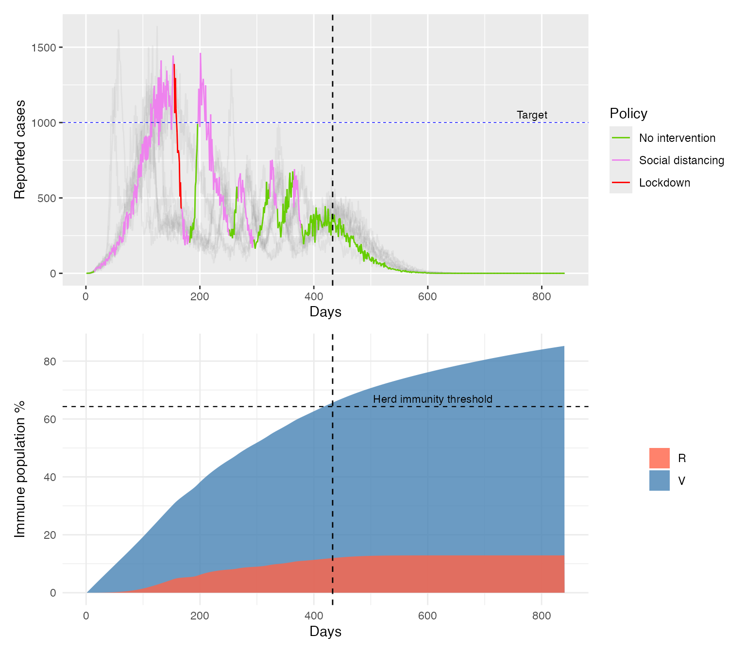
When we plot the results we observe that the controller aims to keep daily incidence near the target level. We focus on the highlighted realisation, while also showing other epidemic realisations as grey curves to illustrate that, although stochasticity affects the exact trajectory, the overall behaviour remains similar. As immunity in the population builds up, this can be achieved by periods of “social distancing” and no intervention whilst the most stringent measure, “lockdown” is used only once at the beginning when population immunity is low (below 20%). Once herd immunity is reached no further intervention is applied. At this point around 16% of the population has infection acquired immunity (recovered) and another 50% is protected by the vaccine. The oscillations in incidence arise because the controller can only choose between three discrete intervention options and policies are reviewed every 14 days. As a result, it cannot continuously fine-tune transmission to maintain exactly R=1. In addition, reporting delays mean that control actions are based on lagged information, which can lead to responses being applied slightly late.
# Combine Simulation Results
results <- lapply(results, function(df) {
     df$cumsum_interv <- (cumsum((1 - df$R_coeff) * (1-df$V/(df$S+df$II+df$V+df$R)) + df$V/(df$S+df$II+df$V+df$R)))
    df
 })

results_old <- results

# save the interventions applied in scenrio sim_id == 1 for reference.
reference_interv <- results_old[[1]]$cumsum_interv

combined_data <- do.call(rbind, results)

combined_data <- combined_data %>%
  group_by(sim_id, policy) %>%
  arrange(days) %>%
  mutate(group = cumsum(c(1, diff(days) != 1))) %>%
  ungroup()

combined_data <- combined_data %>%
  arrange(sim_id, days, policy)

# show the herd immunity threshold
R0 <- Epi_pars$R0
herd_immunity_threshold <- (1 - 1 / R0) * 100

sim1_data <- combined_data %>%
  filter(sim_id == 1) %>%
  mutate(
    immune_pct = (R + V) * 100 / (S + II + V + R)
  )

# first day herd immunity is reached in sim_id == 1
reach_day <- sim1_data %>%
  filter(immune_pct >= herd_immunity_threshold) %>%
  summarise(reach_day = min(days)) %>%
  pull(reach_day)

policy_labels <- c("1" = "No intervention", "2" = "Social distancing", "3" = "Lockdown")

library(patchwork)

top<-ggplot(combined_data %>% filter(sim_id == 1)) +
  geom_line(data = subset(combined_data, sim_id != 1), aes(x = days, y = C, color = as.factor(sim_id)), alpha = 0.1) +
  geom_line(aes(x = days, y = C, color = factor(policy, labels = policy_labels), group = 1), alpha = 1.0) +
  geom_line(aes(x = days, y = C, color = factor(policy, labels = policy_labels), group = 1), alpha = 1.0, linewidth=0.25) +
  geom_hline(yintercept = C_target, linetype = "dashed", color = "blue", linewidth=0.25) +
  annotate(
  "text",
  x = sim_settings$ndays * 0.9,
  y = C_target,
  label = "Target",
  vjust = -0.5,
  hjust = 0,
  size = 3
) +
  geom_vline(
    xintercept = reach_day,
    linetype = "dashed",
    colour = "black",
    linewidth = 0.5
  ) +
  labs(x = "Days", y = "Reported cases", color = "Policy") +
  scale_color_manual(values = c("No intervention" = "chartreuse3", "Social distancing" = "violet", "Lockdown" = "red")) +
  guides(color = guide_legend(title = "Policy"))

# Top panel
bottom <- ggplot(combined_data %>% filter(sim_id == 1), aes(x = days)) +
  geom_area(aes(y = (R+V)*100 / (S + II + V + R), fill = "V"), alpha = 0.8) +
  geom_area(aes(y = (R)*100 / (S + II + V + R), fill = "R"), alpha = 0.8) +
  labs(
    x = "Days",
    y = "Immune population %",
    fill = NULL
  ) +
  geom_hline(
    yintercept = herd_immunity_threshold,
    linetype = "dashed",
    colour = "black",
    linewidth = 0.4
  ) +
  geom_vline(
    xintercept = reach_day,
    linetype = "dashed",
    colour = "black",
    linewidth = 0.5
  ) +
annotate(
  "text",
  x = sim_settings$ndays * 0.6,
  y = herd_immunity_threshold,
  label = "Herd immunity threshold",
  vjust = -0.5,
  hjust = 0,
  size = 3
) +
  scale_fill_manual(
    values = c(
      "V" = "steelblue",
      "R" = "tomato"
    )
  ) +
  theme_minimal()

top/bottom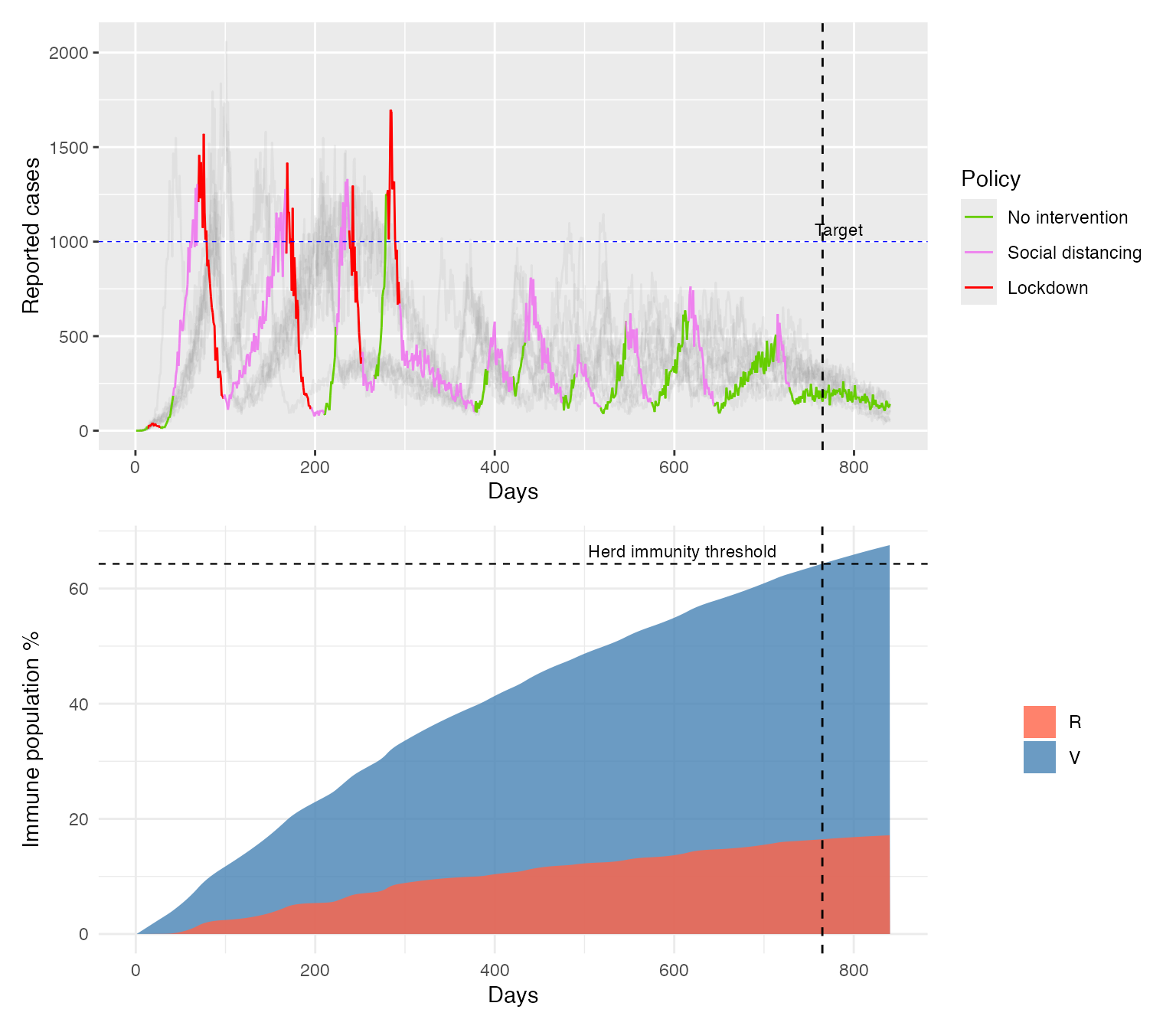
Simulate with a higher vaccination rate
Let’s see what happens if we vaccinate people 2x faster.
model_pars$vac_rate <- Epi_pars$vaccination_rate * 2

episim_data <- data.frame(matrix(0, nrow = (sim_settings$ndays), ncol = length(column_names)))
colnames(episim_data) <- column_names

episim_data$policy <- rep(1, sim_settings$ndays)
episim_data$days <- 1:(sim_settings$ndays)

st0 <- state(model)
episim_data[1, comp_names] <- as.numeric(st0[comp_names])
episim_data[1, "Re"] <- Epi_pars[1, "R0"]
episim_data[1, "Rew"] <- Epi_pars[1, "R0"]
episim_data[1, "R0est"] <- Epi_pars[1, "R0"]
episim_data[1, "Rest"] <- Epi_pars[1, "R0"]
episim_data[1, "I"] <- 1

episim_data_ens <- replicate(sim_settings$sim_ens, episim_data, simplify = FALSE)

for (ii in 1:sim_settings$sim_ens) {
  episim_data_ens[[ii]]$sim_id <- rep(ii, sim_settings$ndays)
}

cl <- makeCluster(Ncores)

clusterExport(cl, ls())
clusterExport(cl, c("reward_fun_wd", "Epi_pred_wd", "Epi_MPC_run_wd", "episim_data_ens", "episettings", "Action_space", "Epi_pars", "Noise_pars", "R_estim"))

parallel::clusterEvalQ(cl, {
  library(pbapply)
  library(VGAM)
  library(EpiControl)
})
#> [[1]]
#>  [1] "EpiControl" "VGAM"       "splines"    "stats4"     "pbapply"
#>  [6] "stats"      "graphics"   "grDevices"  "utils"      "datasets"
#> [11] "methods"    "base"
#>
#> [[2]]
#>  [1] "EpiControl" "VGAM"       "splines"    "stats4"     "pbapply"
#>  [6] "stats"      "graphics"   "grDevices"  "utils"      "datasets"
#> [11] "methods"    "base"

episettings$cl <- cl
episettings$model_par <- model_pars

# Run the epicontrol function
results <- epicontrol(episim_data_ens, episettings)
#> [1] 0
#>   |                                                          |                                                  |   0%

# Stop the cluster after simulation
parallel::stopCluster(cl)
Results
We again simulate an ensemble of 10 scenarios and highlight the one
whose intervention trajectory is closest to the reference case. To
quantify this, we define the metric
cumsum(policy_efficacy * unvaccinated_population + vaccinated_population)
and select the scenario whose resulting trajectory is nearest to the
reference.
We can see that the accelerated vaccination programme leads to a shorter outbreak and roughly a 30% reduction in the total number of infections. With the higher vaccination rate, herd immunity is reached after 430 days rather than around 770, and by that point only around 12% of the population has been infected.
Note that these simulations do not account for vaccination costs, the cumulative burden of infections in the objective function, or any waning of acquired immunity. Nevertheless, they demonstrate how EpiControl can be used for this kind of scenario analysis.
# Combine Simulation Results
results <- lapply(results, function(df) {
     df$cumsum_interv <- (cumsum((1 - df$R_coeff) * (1-df$V/(df$S+df$II+df$V+df$R)) + df$V/(df$S+df$II+df$V+df$R)))
    df
 })

combined_data <- do.call(rbind, results)

combined_data <- combined_data %>%
  group_by(sim_id, policy) %>%
  arrange(days) %>%
  mutate(group = cumsum(c(1, diff(days) != 1))) %>%
  ungroup()

combined_data <- combined_data %>%
  arrange(sim_id, days, policy)

sim1_data <- combined_data %>%
  filter(sim_id == 1) %>%
  mutate(
    immune_pct = (R + V) * 100 / (S + II + V + R)
  )

# first day herd immunity is reached in sim_id == 1
reach_day <- sim1_data %>%
  filter(immune_pct >= herd_immunity_threshold) %>%
  summarise(reach_day = min(days)) %>%
  pull(reach_day)


policy_labels <- c("1" = "No intervention", "2" = "Social distancing", "3" = "Lockdown")

# Here we select the solution thats closest in applied interventions to the reference trajectory
distances <- numeric(length(results))

for (i in 1:sim_settings$n_ens) {
  distances[i] <- sum((results[[i]]$cumsum_interv - reference_interv)^2)
}

best_idx <- which.min(distances)

library(patchwork)

top<-ggplot(combined_data %>% filter(sim_id == best_idx)) +
  geom_line(data = subset(combined_data, sim_id != best_idx), aes(x = days, y = C, color = as.factor(sim_id)), alpha = 0.1) +
  geom_line(aes(x = days, y = C, color = factor(policy, labels = policy_labels), group = 1), alpha = 1.0) +
  geom_line(aes(x = days, y = C, color = factor(policy, labels = policy_labels), group = 1), alpha = 1.0, linewidth=0.25) +
  geom_hline(yintercept = C_target, linetype = "dashed", color = "blue", linewidth=0.25) +
  annotate(
  "text",
  x = sim_settings$ndays * 0.9,
  y = C_target,
  label = "Target",
  vjust = -0.5,
  hjust = 0,
  size = 3
) +
  geom_vline(
    xintercept = reach_day,
    linetype = "dashed",
    colour = "black",
    linewidth = 0.5
  ) +
  labs(x = "Days", y = "Reported cases", color = "Policy") +
  scale_color_manual(values = c("No intervention" = "chartreuse3", "Social distancing" = "violet", "Lockdown" = "red")) +
  guides(color = guide_legend(title = "Policy"))

# Top panel
bottom <- ggplot(combined_data %>% filter(sim_id == best_idx), aes(x = days)) +
  geom_area(aes(y = (R+V)*100 / (S + II + V + R), fill = "V"), alpha = 0.8) +
  geom_area(aes(y = (R)*100 / (S + II + V + R), fill = "R"), alpha = 0.8) +
  labs(
    x = "Days",
    y = "Immune population %",
    fill = NULL
  ) +
  geom_hline(
    yintercept = herd_immunity_threshold,
    linetype = "dashed",
    colour = "black",
    linewidth = 0.4
  ) +
  geom_vline(
    xintercept = reach_day,
    linetype = "dashed",
    colour = "black",
    linewidth = 0.5
  ) +
annotate(
  "text",
  x = sim_settings$ndays * 0.6,
  y = herd_immunity_threshold,
  label = "Herd immunity threshold",
  vjust = -0.5,
  hjust = 0,
  size = 3
) +
  scale_fill_manual(
    values = c(
      "V" = "steelblue",
      "R" = "tomato"
    )
  ) +
  theme_minimal()

top/bottom